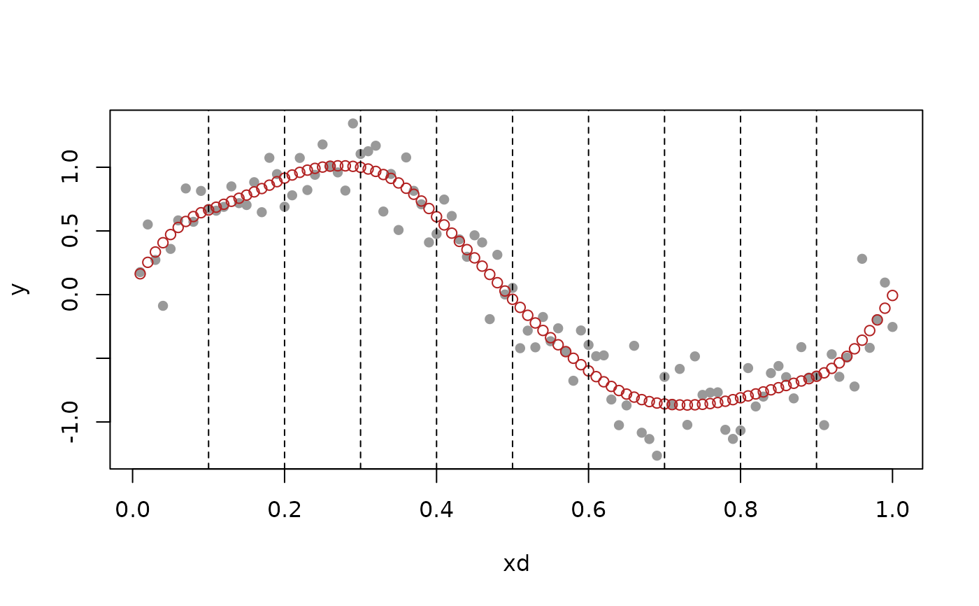
Projects a sequence of values onto the space of discrete splines a given order, with respect to given design points, and given knot points.
Usage
dspline_solve(v, k, xd, knot_idx, basis = c("N", "B", "H"), mat)Arguments
- v
Vector to be values to be projected, one value per design point.
- k
Order for the discrete spline space. Must be >= 0.
- xd
Design points. Must be sorted in increasing order, and have length at least
k+1.- knot_idx
Vector of indices, a subset of
(k+1):(n-1)wheren = length(xd), that indicates which design points should be used as knot points for the discrete spline space. Must be sorted in increasing order.- basis
String, one of
"N","B", or"H", indicating which basis representation is to be used for the least squares computation. The default is"N", the discrete B-spline basis. See details for more information.- mat
Matrix to use for the least squares computation. If missing, the default, then the matrix will be formed according to the
basisargument. See details for more information.
Value
List with components sol: the least squares solution; fit: the
least squares fit; and mat: the basis matrix used for the least squares
problem (only present if the input argument mat is missing).
Details
This function minimizes the least squares criterion
$$
\|v - M \beta\|_2^2
$$
over coefficient vectors \(\beta\); that is, it computes
$$
\hat\beta = (M^T M)^{-1} M^T v
$$
for a vector \(v\) and basis matrix \(M\). The basis matrix \(M\) is
specified via the basis argument, which allows for three options. The
default is "N", in which case the discrete B-spline basis matrix from
n_mat() is used, with the knot_idx argument set accordingly. This is
generally the most stable and efficient option: it leads to a banded,
well-conditioned linear system. Bandedness means that the least squares
projection can be computed in \(O(nk^2)\) operations. See Section 8.4 of
Tibshirani (2020) for numerical experiments investigating conditioning.
The option "H" means that the falling factorial basis matrix from h_mat()
is used, with the col_idx argument set appropriately. This option should
be avoided in general since it leads to a linear system that is neither
sparse nor well-conditioned.
The option "B" means that the extended discrete derivative matrix from
b_mat(), with tf_weighting = TRUE, is used to compute the least squares
solution from projecting onto the falling factorial basis. The fact this is
possible stems from a special inverse relationship between the discrete
derivative matrix and the falling factorial basis matrix. While this option
leads to a banded linear system, this system tends to have worse
conditioning than that using the discrete B-spline representation. However,
it is essentially always preferable to the "H" option, and it produces
the same solution (coefficients in the falling factorial basis expansion).
Note 1: the basis matrix to be used in the least squares problem can be
passed in directly via the mat argument (which saves on the cost of
computing it in the first place). Even when mat not missing, the basis
argument must still be used to specify which type of basis matrix is being
passed in, as the downstream computations differ depending on the type.
Note 2: when mat is not missing and basis = "B", the matrix being
passed in must be the entire extended discrete derivative matrix, as
returned by b_mat() with row_idx = NULL (the default), and not some
row-subsetted version. This is because both the rows corresponding to the
knots in the discrete spline space and the complementary set of roles play
a role in computing the solution. See Section 8.1 of Tibshirani (2020).
References
Tibshirani (2020), "Divided differences, falling factorials, and discrete splines: Another look at trend filtering and related problems", Sections 8.1 and 8.4.
See also
dspline_interp() for interpolation within the "canonical" space of
discrete splines.
